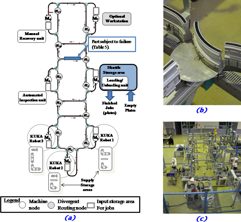
The machines are connected using a transportation system. The transportation system is a one-direction monorail system with rotating transfer gates at routing nodes (Montech, 2011). This transportation system can be considered as a directed, strongly-connected graph, composed of the following nodes:

• M1, M2, M3, M4, M5, M6, M7 (white nodes in below) are the machine nodes,  and
• n1, n2, n3, n4, n5, n6, n7, n8, n9, n10, n11 (gray nodes in below) are divergent routing nodes in which routing decisions must be made (e.g., from n11, it is possible to reach the adjacent nodes n1 or M7).

Shuttles and shuttle storage area

Shuttles are self-propelled transportation resources that transport a job from node to node (Figure 4a). A maximum of 10 shuttles are available. At each moment, a maximum of 10 jobs can be manufactured at the same time (constraints 18-21 in the MILP). Each shuttle embeds a basic behavior to avoid colliding with other shuttles, detect a transfer gate (i.e., stop-and-go system), manage speed in curves and in strait lines, and dock in front of the machines. Because of the technological solution adopted for conveyance, shuttles are governed according to a FIFO rule.

For simplification purposes, it is assumed that empty shuttles are stored in a specific area near the machine M1, with unlimited storage capacity. They enter and leave the cell there. Empty shuttles are loaded with the plates (operation #1) when desired on M1 before entering the cell, go to production and then return to M1 where they are unloaded for delivery. Next, they return in this empty shuttle storage area near M1 until their next use. Thus, there is no possible empty trip in the cell; in the cell, a shuttle has always a job embedded on it.

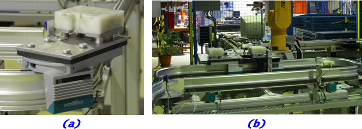
In before, (a) Shuttle with an empty plate and (b) two queued shuttles in the job input storage area of a machine

Job input Storage areas

Before each machine stands a job input storage area with limited capacity, excluding the operating area in front of the machines (Figure 4b). This capacity is set in the cell for one shuttle for all machines (constraint 17 in the MILP). More than one shuttle in the input storage area is risky since it may lock the transportation system for other products and block transfer gates by parking onthem. Specific rules must be designed to handle this situation (e.g., shuttles must keep moving in the central loop until a place is free). Despite this, this value can be increased for simulation or theoretical studies, but not for real experimental studies. The transfer time between the job input storage area and the machine corresponds to the time has the shuttle to move from the storage area and to dock in front of the machine. This time is neglected for all the machines.

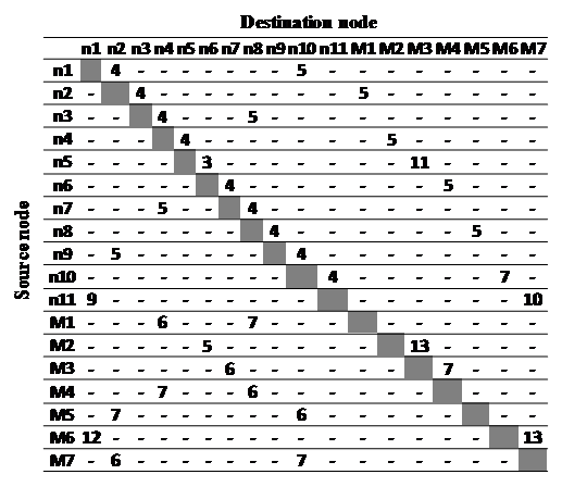
Theoretical transportation times

Table in below shows the theoretical transportation time that is associated to each couple of adjacent nodes. This time is called theoretical since it depends on the actual speed of shuttles. In fact, in reality, a transportation process may last longer that this time due to unexpected events or jamming phenomena.

Data set and objective functions

Given a formal generic model of the target flexible job-shop system, this section tries to define the reference scenario #0 to be chosen by the researchers for the whole benchmark. In this scenario, all the data is known initially. In other words, there are no perturbations. In scenario #0, there is no quality problem, and 100% of the jobs pass inspection. Thus, machine M6 (i.e., recovery) must never be used in the static scenarios.

To design the scenario #0, the researchers must choose a data set, fixing two parameters: 1) the set of client orders, eventually with due dates, and 2) the constraints to be handled. In addition to this data set, the objective function, or performance function, must be determined. Table 4 presents the proposed different data sets. Data sets, in which the constraints are relaxed (e.g., infinite number of shuttles and/or infinite storage capacity and/or neglected transportation times), can be used to obtain bounds or to test basic optimization mechanisms. If the number of shuttles is assumed infinite, then constraints 18-21 in MILP should be relaxed. If the input storage capacity is assumed infinite, then it is constraint 17 that needs to be relaxed. Finally, if transportation times are neglected, then constraints 6 & 7 need to be relaxed.If a due-date-based strategy is chosen, the objective function will be different from the makespan; thus, constraints 22 and 23 should be considered in this case.

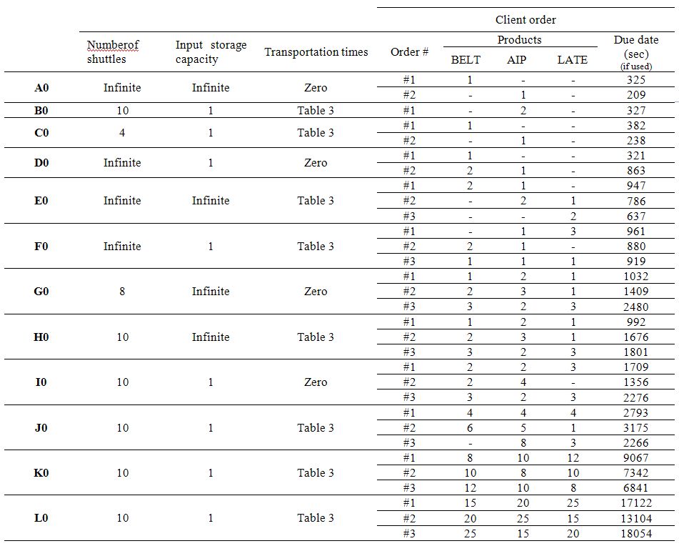
For researchers who pay attention to due-date based production, desired due dates for client orders are provided in the last column of Table 4. These dates have been fine-tuned according to the possible constraint relaxation that may lead to shorten production delays. The problem to be solved has to provide an accurate value for these due dates. As Gordon et al. (2002) noted, there are quite few results on flow and job shop with due-date assignment, and most of the papers are on single and parallel machine shops. Most studies on due-date based scheduling assume uniform distribution of due dates. However, in real production system, this assumption does not always hold true (Thiagarajan and Rajendran, 2005). Sourd (2005) presented a different method for generating due dates that defines the interval bounds in which due dates belong. Those bounds, or range factors, try to control the tightness and variance of due dates. This technique was used by many other authors, for example, Cho and Lazaro (2010). Obviously, the model’s objective function that takes into account due dates must logically take into consideration tardiness or earliness of products.

For researchers who do not pay attention to due dates, these dates can be ignored, and other traditional criteria (e.g., Cmax) can be used.At the designer’s discretion, new scenario can be designed, and a combination of these quantitative indicators or a multicriteria analysis can be performed.

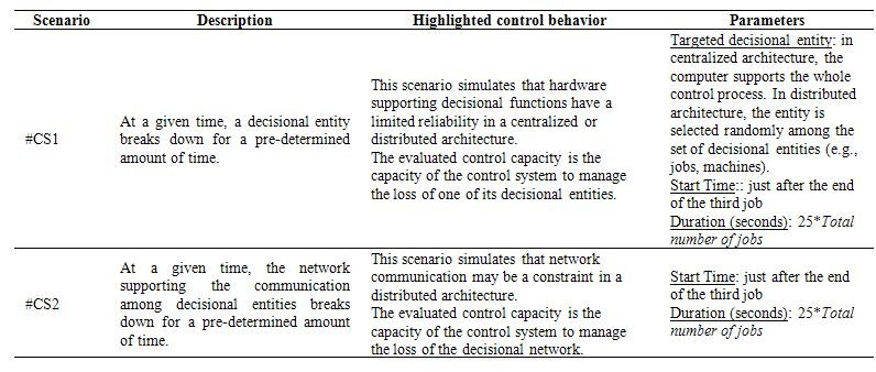
The dynamic scenario list

If testing the dynamic scenarios, several dynamic scenarios must be chosen to evaluate the control system in case of unexpected events. Tables 5 and 6 give a list of dynamic scenarios, numbered according to the increasing complexity level.

In Table 5, dynamic scenarios concern the perturbation of the production system;

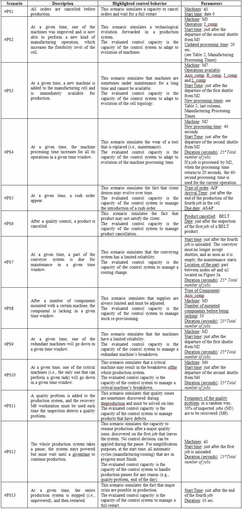
Table 6 provides the dynamic scenarios related to the perturbation of the control system itself.

Obviously, researchers can introduce new scenarios or use these scenarios with different parameters. Otherwise, this list can be considered as a reference list for future comparisons.

Please refer to the publication to see the different data sets and the dynamic scenario list.